
Life expectancy prediction using XGBoost
This project aims to predict the life expectancy of individuals based on a range of health and lifestyle factors. By analyzing data that includes variables such as age, weight, sex, height, systolic blood pressure, smoking habits, use of other nicotine products, and the number of medications taken, the goal is to identify patterns that can help estimate life expectancy. The dataset includes both male and female participants, capturing diverse health profiles across different ages. By building a predictive model, this project hopes to provide insights into how lifestyle choices and medical factors impact longevity, ultimately contributing to better health predictions and personalized healthcare interventions.
Data Source: url=“https://www.kaggle.com/datasets/joannpineda/individual-age-of-death-and-related-factors/data”
# Import the libraries
import pandas as pd
import numpy as np
import json
import matplotlib.pyplot as plt
import seaborn as sns
## Read the json file into pandas datarame
df=pd.read_json('data.json')
Data Preprocessing
1. Handle Missing values
# Check for missing values in the dataset
print("Missing Values:\n", df.isnull().sum())
Missing Values:
 age                     0
weight                  0
sex                     0
height                  0
sys_bp                  0
smoker                  0
nic_other               0
num_meds                0
occup_danger            0
ls_danger               0
cannabis                0
opioids                 0
other_drugs             0
drinks_aweek            0
addiction               0
major_surgery_num       0
diabetes                0
hds                     0
cholesterol             0
asthma                  0
immune_defic            0
family_cancer           0
family_heart_disease    0
family_cholesterol      0
dtype: int64
The dataset doesnot contain any missing or null values
2. Feature Engineering
# create BMI feature on weight and height:
df['bmi'] = df['weight'] / (df['height'] ** 2) * 703  # if height is in inches and weight is in pounds
3. Convert Categorical variables to Numerical variables
# Check the data types of each column to identify categorical variables
categorical_columns = df.select_dtypes(include=['object']).columns.tolist()

# Display the list of categorical columns
print("Categorical Columns:", categorical_columns)
Categorical Columns: ['sex', 'smoker', 'nic_other', 'cannabis', 'opioids', 'other_drugs', 'addiction', 'diabetes', 'hds', 'asthma', 'immune_defic', 'family_cancer', 'family_heart_disease', 'family_cholesterol']
The categorical variables are binary, so I have used label encoding (0-‘y’,1-‘n’) or (0-‘f’,1-‘m’)
# Convert categorical columns to numeric
df['sex'] = df['sex'].map({'m': 1, 'f': 0})
df['smoker'] = df['smoker'].map({'n': 0, 'y': 1})
df['cannabis'] = df['cannabis'].map({'n': 0, 'y': 1})
df['nic_other'] = df['nic_other'].map({'n': 0, 'y': 1})
df['opioids'] = df['opioids'].map({'n': 0, 'y': 1})
df['other_drugs'] = df['other_drugs'].map({'n': 0, 'y': 1})
df['addiction'] = df['addiction'].map({'n': 0, 'y': 1})
df['hds'] = df['hds'].map({'n': 0, 'y': 1})
df['diabetes'] = df['diabetes'].map({'n': 0, 'y': 1})
df['asthma'] = df['asthma'].map({'n': 0, 'y': 1})
df['immune_defic'] = df['immune_defic'].map({'n': 0, 'y': 1})
df['family_cancer'] = df['family_cancer'].map({'n': 0, 'y': 1})
df['family_heart_disease'] = df['family_heart_disease'].map({'n': 0, 'y': 1})
df['family_cholesterol'] = df['family_cholesterol'].map({'n': 0, 'y': 1})
In this project, I am applying XGBoost model for the prediction so, I am not applying feature scaling on the numerical variables. ince XGBoost is a tree-based algorithm, feature scaling is not necessary for the numerical variables. Tree-based models like XGBoost work by splitting the data at specific values (thresholds) of the features to make decisions, rather than relying on distances between data points, as seen in distance-based algorithms like KNN or SVM. Because of this, the scale of the numerical features does not affect the performance of the model. Therefore, I will skip the feature scaling step for the numerical variables in this analysis.
4. Target variable distribution
plt.figure(figsize=(8,5))
sns.histplot(df['age'], bins=20, kde=True)
plt.title("Age at Death Distribution")
plt.show()
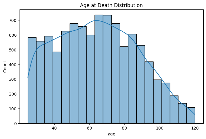
I wanted to see if the distribution of target variable is skewed i.e. if the dataset has similar age at death, the model might be biased towards mean or median. In such case, we have to consider applying log transformation of the target variable. However, after plotting the distribution, I observed that age at death is slightly right-skewed, indicating that the mean age is marginally higher than the median. Given this slight skew, I have decided not to apply a log transformation to the target variable, as the skewness is not severe enough to warrant a transformation that would distort the data.
Model Training (XGBoost Model)
1. Test Train Split
from sklearn.model_selection import train_test_split

# Assuming the target variable is 'estimated_lifespan'
X = df.drop(columns=['age','weight','height'])  # Features
y = df['age']  # Target variable

# Split the data into training and testing sets (80% train, 20% test)
X_train, X_test, y_train, y_test = train_test_split(X, y, test_size=0.2, random_state=42)

print(f"Training data: {X_train.shape}, Test data: {X_test.shape}")
Training data: (8000, 22), Test data: (2000, 22)
2. Model Training and Prediction
!pip install xgboost
import xgboost as xgb
from sklearn.metrics import mean_absolute_error, mean_squared_error, r2_score
model = xgb.XGBRegressor(
    n_estimators=100,  # Number of boosting rounds (trees)
    learning_rate=0.1,  # Step size shrinkage to prevent overfitting
    max_depth=6,  # Maximum depth of each tree
    objective='reg:squarederror',  # Objective function for regression
    random_state=42
)

# Train the model
model.fit(X_train, y_train)
XGBRegressor(base_score=None, booster=None, callbacks=None,
             colsample_bylevel=None, colsample_bynode=None,
             colsample_bytree=None, device=None, early_stopping_rounds=None,
             enable_categorical=False, eval_metric=None, feature_types=None,
             gamma=None, grow_policy=None, importance_type=None,
             interaction_constraints=None, learning_rate=0.1, max_bin=None,
             max_cat_threshold=None, max_cat_to_onehot=None,
             max_delta_step=None, max_depth=6, max_leaves=None,
             min_child_weight=None, missing=nan, monotone_constraints=None,
             multi_strategy=None, n_estimators=100, n_jobs=None,
             num_parallel_tree=None, random_state=42, ...)
In a Jupyter environment, please rerun this cell to show the HTML representation or trust the notebook. On GitHub, the HTML representation is unable to render, please try loading this page with nbviewer.org.
XGBRegressor(base_score=None, booster=None, callbacks=None,
             colsample_bylevel=None, colsample_bynode=None,
             colsample_bytree=None, device=None, early_stopping_rounds=None,
             enable_categorical=False, eval_metric=None, feature_types=None,
             gamma=None, grow_policy=None, importance_type=None,
             interaction_constraints=None, learning_rate=0.1, max_bin=None,
             max_cat_threshold=None, max_cat_to_onehot=None,
             max_delta_step=None, max_depth=6, max_leaves=None,
             min_child_weight=None, missing=nan, monotone_constraints=None,
             multi_strategy=None, n_estimators=100, n_jobs=None,
             num_parallel_tree=None, random_state=42, ...)
# Predict on the test set
y_pred = model.predict(X_test)
# Calculate evaluation metrics
mae = mean_absolute_error(y_test, y_pred)
mse = mean_squared_error(y_test, y_pred)
rmse = mean_squared_error(y_test, y_pred, squared=False)
r2 = r2_score(y_test, y_pred)
print(f"Mean Absolute Error (MAE): {mae}")
print(f"Mean Squared Error (MSE): {mse}")
print(f"Root Mean Squared Error (RMSE): {rmse}")
print(f"R-squared (R²): {r2}")
Mean Absolute Error (MAE): 11.245285104751586
Mean Squared Error (MSE): 197.77419800935633
Root Mean Squared Error (RMSE): 14.063221466269963
R-squared (R²): 0.6389341600450889
Mean Absolute Error (MAE) represents the average absolute difference between the predicted and actual values. An MAE of 11.24 indicates that, on average, the model’s predictions are off by 11.24 years. Mean Squared Error (MSE) measures the average of the squared differences between the predicted and actual values. Root Mean Squared Error (RMSE) provides an indication of how much the model’s predictions deviate from the actual values. An RMSE of 14.06 suggests that, on average, the model’s predictions are off by approximately 14.06 years.
I am using RMSE as the evaluation metric because age is a continuous variable, and RMSE better reflects the model’s performance by penalizing larger errors. R-squared (R²) measures the proportion of variance in the target variable (age) that is explained by the model. An R-squared value of 0.6389 means that the model explains about 63.89% of the variance in age.
3. Model Tuning
Since R-squared is 63.89%, I want to optimize the model’s hyperparameters to improve it’s performance. I am using Grid Search method to define a combination of hyperparameters to find the best performing set.
from sklearn.model_selection import GridSearchCV

# Set up the parameter grid for hyperparameter tuning

params =  {
    'max_depth': [3, 5, 6, 7],
    'learning_rate': [0.05, 0.1, 0.2],
    'n_estimators': [100, 500, 1000],
    'subsample': [0.8, 1.0],  # Sampling fraction
    'colsample_bytree': [0.8, 1.0]  # Feature selection
}
# Initialize GridSearchCV
grid_search = GridSearchCV(estimator=model, param_grid=params, cv=5, scoring='r2')

# Fit GridSearchCV
grid_search.fit(X_train, y_train)

# Get the best hyperparameters
best_params = grid_search.best_params_
print(f"Best Hyperparameters: {best_params}")

# Retrain the model with the best parameters
best_model = grid_search.best_estimator_

# Evaluate the best model
y_pred_best = best_model.predict(X_test)

# Calculate evaluation metrics for the best model
mae_best = mean_absolute_error(y_test, y_pred_best)
mse_best = mean_squared_error(y_test, y_pred_best)
rmse_best = mean_squared_error(y_test, y_pred_best, squared=False)
r2_best = r2_score(y_test, y_pred_best)

print(f"Best Model - Mean Absolute Error (MAE): {mae_best}")
print(f"Best Model - Mean Squared Error (MSE): {mse_best}")
print(f"Best Model - Root Mean Squared Error (RMSE): {rmse_best}")
print(f"Best Model - R-squared (R²): {r2_best}")
Best Hyperparameters: {'colsample_bytree': 0.8, 'learning_rate': 0.05, 'max_depth': 3, 'n_estimators': 500, 'subsample': 0.8}
Best Model - Mean Absolute Error (MAE): 11.045282677650452
Best Model - Mean Squared Error (MSE): 190.53224406528577
Best Model - Root Mean Squared Error (RMSE): 13.803341771661158
Best Model - R-squared (R²): 0.6521554103904292
After performing hyperparameter tuning, the model performance improved by 1.32%
4. Residual Test
Since, the model performance didnot improve even after hyperparameter tuning, I want to see how well the model fits the data. For that, I will perform residual test analysis on train and test set.
y_train_best = best_model.predict(X_train)
residuals_train = y_train - y_train_best
residuals_test = y_test - y_pred_best

plt.scatter(y_train_best, residuals_train)
plt.axhline(y=0, color='r', linestyle='--')
plt.xlabel("Predicted Age at Death")
plt.ylabel("Residuals vs Predicted (Training Data)")
plt.title("Residual Plot")
plt.show()


plt.scatter(y_pred_best, residuals_test)
plt.axhline(y=0, color='r', linestyle='--')
plt.xlabel("Predicted Age at Death")
plt.ylabel("Residuals vs Predicted (Test Data)")
plt.title("Residual Plot")
plt.show()
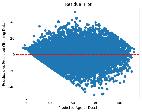
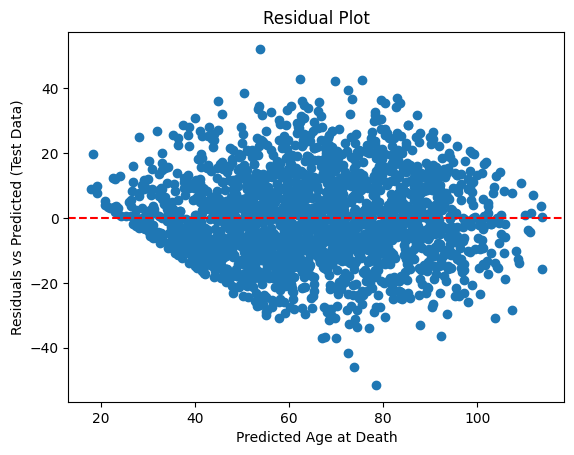
From the residual plot, we can see the residuals are widely scattered around zero, forming a funnel shape for both train and test set. This suggests heteroscedasticity, i.e. the variance of residuals increases as the predicted age increases. The shape of the residuals in the test set is similar to the training set, suggesting the model has generalized reasonably well and the model is not heavily overfitted.
4. Model Evaluation
# Get feature importances from XGBoost
# Method 1: Using the built-in `feature_importances_` (similar to RandomForest)
feature_importances = best_model.feature_importances_

# Method 2: Using the booster object to get feature importance with different importance types (e.g., weight, gain)
booster = best_model.get_booster()

# Calculate feature importances
importance = booster.get_score(importance_type='weight')
importance_df = pd.DataFrame({
    'feature': list(importance.keys()),
    'importance': list(importance.values())
}).sort_values(by='importance', ascending=False)

# Display the importance dataframe
print(importance_df)
feature importance
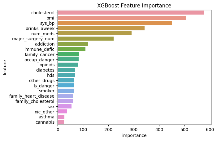
15 cholesterol 576.0
21 bmi 505.0
1 sys_bp 450.0
10 drinks_aweek 343.0
4 num_meds 291.0
12 major_surgery_num 221.0
11 addiction 120.0
17 immune_defic 110.0
18 family_cancer 84.0
5 occup_danger 83.0
8 opioids 80.0
13 diabetes 69.0
14 hds 69.0
9 other_drugs 64.0
6 ls_danger 63.0
2 smoker 63.0
19 family_heart_disease 61.0
20 family_cholesterol 60.0
0 sex 55.0
3 nic_other 37.0
16 asthma 27.0
7 cannabis 24.0
# Create a bar plot for feature importances
sns.barplot(x='importance', y='feature', data=importance_df)
plt.title('XGBoost Feature Importance')
plt.show()
# Test the model on sample data
sample1 = [[120, 0, 0, 0, 0, 0, 125, 29.0, 1, 0, 0, 0, 0, 0, 0, 0, 0, 0, 1, 1, 1, 1]]
sample2 = [[180, 5, 1, 1, 15, 2, 280, 35.0, 1, 1, 1, 1, 1, 1, 1, 1, 1, 1, 0, 0, 1, 1]]
sample3 = [[150, 3, 0, 0, 10, 1, 180, 30.0, 0, 0, 2, 1, 1, 0, 0, 0, 1, 0, 1, 1, 0, 1]]
sample4 = [[110, 2, 2, 2, 5, 6, 125, 28.0, 1, 1, 1, 1, 1, 0, 0, 0, 0, 0, 1, 1, 1, 1]]
sample5 = [[160, 4, 1, 1, 12, 1, 200, 32.0, 0, 0, 1, 1, 0, 1, 1, 1, 0, 0, 0, 1, 1, 1]]

# Prediction of the age at death based on best_model
print(round(best_model.predict(sample1)[0]))
print(round(best_model.predict(sample2)[0]))
print(round(best_model.predict(sample3)[0]))
print(round(best_model.predict(sample4)[0]))
print(round(best_model.predict(sample5)[0]))
97
42
74
71
65
Model implementation on user input data
# Function to get user input for the features in model
def get_user_input():

    sys_bp = int(input("Enter systolic blood pressure level (sys_bp): "))
    num_meds = int(input("Enter number of medications: "))
    occup_danger = int(input("Is your occupation dangerous? ('0' for low, '1' for medium, '2' for high): "))
    ls_danger = int(input("Is your lifestyle dangerous? ('0' for low, '1' for medium, '2' for high): "))
    drinks_aweek = int(input("How many drinks you drink per week?: "))
    major_surgery_num = int(input("Enter number of major surgeries: "))
    cholesterol = int(input("Enter your cholesterol level: "))
    bmi = float(input("Enter BMI: "))
    sex = str(input("Enter your gender ('m' for male and 'f' for female): "))
    smoker = str(input("Do you smoke? ('y' for Yes, 'n' for No): "))
    nic_other = str(input("Do you use any other form of nicotine? ('y' for Yes, 'n' for No): "))
    cannabis = str(input("Do you use cannabis? ('y' for Yes, 'n' for No): "))
    opioids = str(input("Do you use opioids? ('y' for Yes, 'n' for No): "))
    other_drugs = str(input("Do you use other drugs? ('y' for Yes, 'n' for No): "))
    addiction = str(input("Do you have any form of addiction? ('y' for Yes, 'n' for No): "))
    diabetes = str(input("Do you have diabetes? ('y' for Yes, 'n' for No): "))
    hds = str(input("Do you have any health disease? ('y' for Yes, 'n' for No): "))
    asthma = str(input("Do you have asthma? ('y' for Yes, 'n' for No): "))
    immune_defic = str(input("Do you have any immune deficiency? ('y' for Yes, 'n' for No): "))
    family_cancer = str(input("Do you have a family history of cancer? ('y' for Yes, 'n' for No): "))
    family_heart_disease = str(input("Do you have a family history of heart disease? ('y' for Yes, 'n' for No): "))
    family_cholesterol = str(input("Do you have a family history of cholesterol? ('y' for Yes, 'n' for No): "))


     # Store the responses in a dictionary
    user_input = {
        'sys_bp': sys_bp,               # Systolic blood pressure
        'num_meds': num_meds,           # Number of medications
        'occup_danger': occup_danger,   # Occupation danger level
        'ls_danger': ls_danger,         # Lifestyle danger level
        'drinks_aweek': drinks_aweek,   # Number of drinks per week
        'major_surgery_num': major_surgery_num,  # Number of major surgeries
        'cholesterol': cholesterol,     # Cholesterol level
        'bmi': bmi,                     # Body Mass Index
        'sex': sex,                     # Gender ('m' for male, 'f' for female)
        'smoker': smoker,               # Smoking status ('y' for Yes, 'n' for No)
        'nic_other': nic_other,         # Use of other forms of nicotine ('y' for Yes, 'n' for No)
        'cannabis': cannabis,           # Cannabis use ('y' for Yes, 'n' for No)
        'opioids': opioids,             # Opioid use ('y' for Yes, 'n' for No)
        'other_drugs': other_drugs,     # Use of other drugs ('y' for Yes, 'n' for No)
        'addiction': addiction,         # Addiction status ('y' for Yes, 'n' for No)
        'diabetes': diabetes,           # Diabetes status ('y' for Yes, 'n' for No)
        'hds': hds,                     # Health disease status ('y' for Yes, 'n' for No)
        'asthma': asthma,               # Asthma status ('y' for Yes, 'n' for No)
        'immune_defic': immune_defic,   # Immune deficiency status ('y' for Yes, 'n' for No)
        'family_cancer': family_cancer, # Family history of cancer ('y' for Yes, 'n' for No)
        'family_heart_disease': family_heart_disease, # Family history of heart disease ('y' for Yes, 'n' for No)
        'family_cholesterol': family_cholesterol  # Family history of cholesterol ('y' for Yes, 'n' for No)
    }

    # Print the responses with respective questions
    print("\nUser Responses:")
    for question, response in user_input.items():
        print(f"{question.replace('_', ' ').title()}: {response}")

    return user_input
# Function to preprocess user input data
def preprocess_input(user_input):
    # Convert user input to a DataFrame
    input_df = pd.DataFrame([user_input], columns=[
        'sys_bp', 'num_meds', 'occup_danger', 'ls_danger', 'drinks_aweek' ,
            'major_surgery_num','cholesterol', 'bmi', 'sex', 'smoker', 'nic_other','cannabis',
                'opioids', 'other_drugs', 'addiction', 'diabetes', 'hds', 'asthma', 'immune_defic',
                    'family_cancer', 'family_heart_disease', 'family_cholesterol'
    ])


    # Check the data types of each column to identify categorical variables
    categorical_cols = input_df.select_dtypes(include=['object']).columns.tolist()

    df_input_encoded = pd.get_dummies(input_df, columns=categorical_cols)

     # Ensure all the columns are in the same order as the model expects
    df_input_encoded = df_input_encoded.reindex(columns=model.get_booster().feature_names, fill_value=0)

    return df_input_encoded
# Main program
user_input = get_user_input()
processed_input = preprocess_input(user_input)

# Predict the age at death based on the user's input
predicted_age = best_model.predict(processed_input)

print(f"The predicted age at death is: {round(predicted_age[0])}")
User Responses:
Sys Bp: 120
Num Meds: 4
Occup Danger: 4
Ls Danger: 0
Drinks Aweek: 4
Major Surgery Num: 1
Cholesterol: 120
Bmi: 31.0
Sex: m
Smoker: n
Nic Other: y
Cannabis: y
Opioids: n
Other Drugs: n
Addiction: n
Diabetes: y
Hds: n
Asthma: y
Immune Defic: n
Family Cancer: y
Family Heart Disease: n
Family Cholesterol: y
Index(['sex', 'sys_bp', 'smoker', 'nic_other', 'num_meds', 'occup_danger',
       'ls_danger', 'cannabis', 'opioids', 'other_drugs', 'drinks_aweek',
       'addiction', 'major_surgery_num', 'diabetes', 'hds', 'cholesterol',
       'asthma', 'immune_defic', 'family_cancer', 'family_heart_disease',
       'family_cholesterol', 'bmi'],
      dtype='object')
The predicted age at death is: 104