
MMA kick and punch detection
This project focuses on developing a classifier to identify kicks and punches in MMA fights using a dataset consisting of 597 annotated images captured from raw MMA fights using Roboflow. Initially, we trained six models (VGG, Resnet50, InceptionResnetV2, MobileNetV2 , EfficientNetB0 , YoloV8) with four image classes: kick, punch, kicknt (kick no touch), and punchnt (punch no touch). However, these models only achieved an average accuracy of 30%, and despite making various attempts at data augmentation and using different models for training, we couldn’t improve their performance.
To address this issue, we simplified the problem by removing the kicknt and punchnt classes and retrained the six models with just two classes: kick and punch. This modification resulted in a significant improvement, with an average accuracy increase of 30% across all models.
In an effort to further enhance the performance, we decided to experiment with the YoloV8n classification model. To ensure fair comparisons, we conducted experiments using both the original dataset with four classes and the simplified dataset with two classes. These experiments aimed to identify the most suitable model and approach for accurately classifying kicks and punches in MMA fights.
Among the six models we trained, YOLOV8 model was the best performer with the accuracy of 75% and EfficientNET was the least performer with accuracy of 53.12%. We have also created a Streamlit app for kick and punch classifier using YOLOV8 model.
StreamLit URL: https://kick-and-punch-classifier.streamlit.app/
GitHub repository: https://github.com/sirjanashrestha/kick-and-punch-detection
Data
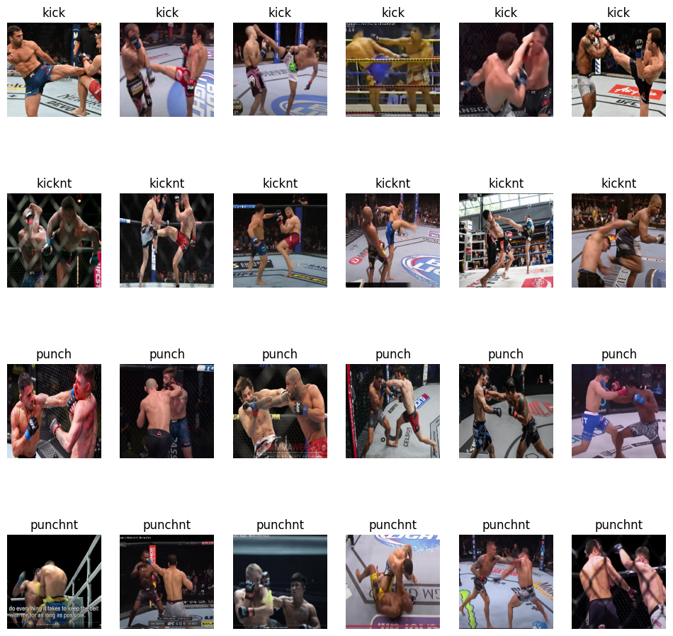
We created a custom dataset from the ground up, immersing ourselves in MMA videos on YouTube capturing screenshots.This comprehensive dataset encompasses four distinct classes: “kick,” “kicknt” (no touch), “punch,” and “punchnt” (no touch).
To expedite the image classification process and optimize dataset division, we used Roboflow tool which helped us to systematically arrange, annotate, and categorize the images.
Tha dataset can be downloaded from: https://universe.roboflow.com/georgebrown/punch-and-kick-detection-group
Our dataset and classes
# Number of samples per class to display
num_samples_per_class = 6

# Function to display sample images from each class
def show_sample_images(data_dir, classes, num_samples_per_class):
    plt.figure(figsize=(12,12))

    for i, class_name in enumerate(classes):
        class_dir = os.path.join(data_dir, class_name)
        class_images = random.sample(os.listdir(class_dir), num_samples_per_class)

        for j, image_name in enumerate(class_images):
            image_path = os.path.join(class_dir, image_name)
            image = load_img(image_path, target_size=(weight_size, height_size))

            plt.subplot(len(classes), num_samples_per_class, i * num_samples_per_class + j + 1)
            plt.imshow(image)
            plt.title(class_name)
            plt.axis('off')

    plt.show()

# Call the function to show sample images from each class
show_sample_images(train_path, classes, num_samples_per_class)
Methods
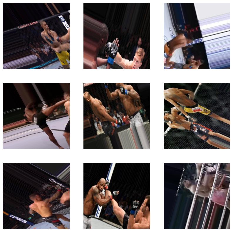
Our dataset with data augmentation
train_datagen = ImageDataGenerator(
    rescale=1.0 / 255,           # Normalize pixel values to [0,1]
    rotation_range=90,           # Randomly rotate images by up to 20 degrees
    width_shift_range=0.4,       # Randomly shift images horizontally by up to 20% of the width
    height_shift_range=0.4,      # Randomly shift images vertically by up to 20% of the height
    shear_range=0.5,             # Apply shear transformation
    zoom_range=0.2,              # Randomly zoom images by up to 20%
    horizontal_flip=True,        # Randomly flip images horizontally
    fill_mode='nearest'          # Use the nearest pixel to fill missing areas after augmentation
)
plt.figure(figsize=(10, 10))
images, _ = next(training_set)
for i, image in enumerate(images[: 9]):
    ax = plt.subplot(3, 3, i + 1)
    plt.imshow(image)
    plt.axis('off')
Experiments
First, we trained 6 models with 4 classes
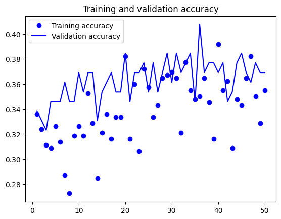
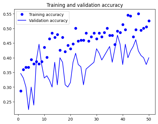
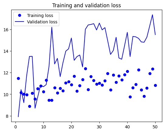
1. VGG16 model with 100.356 trainable params and 14.815.044 total params, no dropout but with data augmentation
#Load the VGG16 model with pre-trained weights
vgg = VGG16(input_shape=IMAGE_SIZE + [3], weights='imagenet', include_top=False)
# freeze the layers
for layer in vgg.layers:
    layer.trainable = False
x = Flatten()(vgg.output)
#x = Dropout(0.5)(x)
#x = Dense(256, activation='relu')(x)

# adding output layer with number of classes = len(folders)
# it is a dense (fully connected) layer with a softmax activation function
prediction = Dense(len(folders), activation='softmax')(x)
vgg_model = Model(inputs=vgg.input, outputs=prediction)
test_model = keras.models.load_model(
    "./models/convnet_vgg_4_classes.keras")
test_loss, test_acc = test_model.evaluate(test_set)
print(f"Test accuracy: {test_acc:.3f}")
accuracy = history.history["accuracy"]
val_accuracy = history.history["val_accuracy"]
loss = history.history["loss"]
val_loss = history.history["val_loss"]
epochs = range(1, len(accuracy) + 1)
plt.plot(epochs, accuracy, "bo", label="Training accuracy")
plt.plot(epochs, val_accuracy, "b", label="Validation accuracy")
plt.title("Training and validation accuracy")
plt.legend()
plt.figure()
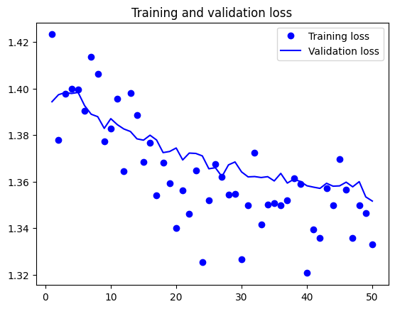
plt.plot(epochs, loss, "bo", label="Training loss")
plt.plot(epochs, val_loss, "b", label="Validation loss")
plt.title("Training and validation loss")
plt.legend()
plt.show()
2. ResNet50V2 with 401.412 trainable parameters and 23.966.212 total params, no dropout but with data augmentation
resnet = ResNet50V2(input_shape=IMAGE_SIZE + [3], weights='imagenet', include_top=False)

#freezing the layers
for layer in resnet.layers[:-1]:
    layer.trainable = False

# defining the final layers of the model.
x = Flatten()(resnet.output)

prediction = Dense(len(folders), activation='softmax')(x)
model = Model(inputs=resnet.input, outputs=prediction)
# definfing the final layers of the model
x = inception.output
x = GlobalAveragePooling2D()(x)
x = Flatten()(x)
x = Dropout(0.5)(x)
x = Dense(512, activation='relu')(x)
predictions = Dense(len(folders), activation='softmax')(x)

model = Model(inputs=inception.input, outputs=predictions)
test_model = keras.models.load_model(
    "./models/convnet_resnet_4_classes.keras")
test_loss, test_acc = test_model.evaluate(test_set)
print(f"Test accuracy: {test_acc:.3f}")
accuracy = history.history["accuracy"]
val_accuracy = history.history["val_accuracy"]
loss = history.history["loss"]
val_loss = history.history["val_loss"]
epochs = range(1, len(accuracy) + 1)
plt.plot(epochs, accuracy, "bo", label="Training accuracy")
plt.plot(epochs, val_accuracy, "b", label="Validation accuracy")
plt.title("Training and validation accuracy")
plt.legend()
plt.figure()
plt.plot(epochs, loss, "bo", label="Training loss")
plt.plot(epochs, val_loss, "b", label="Validation loss")
plt.title("Training and validation loss")
plt.legend()
plt.show()
3. InceptionResNetV2 with 3.985.412 trainable parameters and 55.125.732 total params, with dropout of 0.5, Average Pooling and a fully connect layer
# definfing the final layers of the model
x = inception.output
x = GlobalAveragePooling2D()(x)
x = Flatten()(x)
x = Dropout(0.5)(x)
x = Dense(512, activation='relu')(x)
predictions = Dense(len(folders), activation='softmax')(x)

model = Model(inputs=inception.input, outputs=predictions)
test_model = keras.models.load_model(
    "./models/convnet_inceptionResnet_4_classes.keras")
test_loss, test_acc = test_model.evaluate(test_set)
print(f"Test accuracy: {test_acc:.3f}")
accuracy = history.history["accuracy"]
val_accuracy = history.history["val_accuracy"]
loss = history.history["loss"]
val_loss = history.history["val_loss"]
epochs = range(1, len(accuracy) + 1)
plt.plot(epochs, accuracy, "bo", label="Training accuracy")
plt.plot(epochs, val_accuracy, "b", label="Validation accuracy")
plt.title("Training and validation accuracy")
plt.legend()
plt.figure()
plt.plot(epochs, loss, "bo", label="Training loss")
plt.plot(epochs, val_loss, "b", label="Validation loss")
plt.title("Training and validation loss")
plt.legend()
plt.show()
4. MobileNETV2 with 726,820 trainable parameters and 2,985,828 total parameters, with dropout of 0.3, Average Pooling and a fully connected layer
# creating a new sequential model using a pre-trained MobileNetV2
tf.keras.backend.clear_session()

model = Sequential([mnet,
                    GlobalAveragePooling2D(),
                    Dense(512, activation = "ReLU"),
                    BatchNormalization(),
                    Dropout(0.3),
                    Dense(128, activation = "ReLU"),
                    Dropout(0.1),
                    Dense(32, activation = "ReLU"),
                    Dropout(0.3),
                    Dense(4, activation = "sigmoid")])

model.layers[0].trainable = False

model.compile(loss="categorical_crossentropy", optimizer="Adam", metrics="accuracy")

model.summary()
Model: "sequential"
Model: "sequential"
_________________________________________________________________
 Layer (type)                Output Shape              Param #
=================================================================
 mobilenetv2_1.00_224 (Funct  (None, 7, 7, 1280)       2257984
 ional)

 global_average_pooling2d (G  (None, 1280)             0
 lobalAveragePooling2D)

 dense (Dense)               (None, 512)               655872

 batch_normalization (BatchN  (None, 512)              2048
 ormalization)

 dropout (Dropout)           (None, 512)               0

 dense_1 (Dense)             (None, 128)               65664

 dropout_1 (Dropout)         (None, 128)               0

 dense_2 (Dense)             (None, 32)                4128

 dropout_2 (Dropout)         (None, 32)                0

 dense_3 (Dense)             (None, 4)                 132

=================================================================
Total params: 2,985,828
Trainable params: 726,820
Non-trainable params: 2,259,008
_________________________________________________________________
test_loss, test_accuracy = model.evaluate_generator(generator = test_set, verbose = 1)

print('Test Accuracy: ', round((test_accuracy * 100), 2), "%")
epochs = 50
train_loss = hist.history['loss']
val_loss = hist.history['val_loss']
train_acc = hist.history['accuracy']
val_acc = hist.history['val_accuracy']
xc = range(epochs)

plt.figure(1,figsize=(7,5))
plt.plot(xc,train_loss)
plt.plot(xc,val_loss)
plt.xlabel('num of Epochs')
plt.ylabel('loss')
plt.title('train_loss vs val_loss')
plt.grid(True)
plt.legend(['train','val'])
#print plt.style.available # use bmh, classic,ggplot for big pictures
plt.style.use(['classic'])

plt.figure(2,figsize=(7,5))
plt.plot(xc,train_acc)
plt.plot(xc,val_acc)
plt.xlabel('num of Epochs')
plt.ylabel('accuracy')
plt.title('train_acc vs val_acc')
plt.grid(True)
plt.legend(['train','val'],loc=4)
#print plt.style.available # use bmh, classic,ggplot for big pictures
plt.style.use(['classic'])
5. EfficientNET with 4,012,672 trainable parameters and 4,054,688 total parameters, with dropout of 0.5, GlobalAveragePooling and a fully connected layer
efnb0 = efn.EfficientNetB0(weights='imagenet', include_top=False, input_shape=(224,224,3), classes=n_classes)

model = Sequential()
model.add(efnb0)
model.add(GlobalAveragePooling2D())
model.add(Dropout(0.5))
model.add(Dense(n_classes, activation='softmax'))

model.summary()
Model: "sequential_1"
_________________________________________________________________
 Layer (type)                Output Shape              Param #
=================================================================
 efficientnet-b0 (Functional  (None, 7, 7, 1280)       4049564
 )

 global_average_pooling2d_1   (None, 1280)             0
 (GlobalAveragePooling2D)

 dropout_3 (Dropout)         (None, 1280)              0

 dense_4 (Dense)             (None, 4)                 5124

=================================================================
Total params: 4,054,688
Trainable params: 4,012,672
Non-trainable params: 42,016
_________________________________________________________________
test_loss, test_accuracy = model.evaluate_generator(generator = test_set, verbose = 1)

print('Test Accuracy: ', round((test_accuracy * 100), 2), "%")
#plot to visualize the loss and accuracy against number of epochs
plt.figure(figsize=(18,8))

plt.suptitle('Loss and Accuracy Plots', fontsize=18)

plt.subplot(1,2,1)
plt.plot(model_history.history['loss'], label='Training Loss')
plt.plot(model_history.history['val_loss'], label='Validation Loss')
plt.legend()
plt.xlabel('Number of epochs', fontsize=15)
plt.ylabel('Loss', fontsize=15)

plt.subplot(1,2,2)
plt.plot(model_history.history['accuracy'], label='Train Accuracy')
plt.plot(model_history.history['val_accuracy'], label='Validation Accuracy')
plt.legend()
plt.xlabel('Number of epochs', fontsize=14)
plt.ylabel('Accuracy', fontsize=14)
plt.show()
6. YoloV8 with 99 layers, 1443412 parameters, 1443412 gradients
model = YOLO('yolov8n-cls.pt') # load a pretrained model (recommended for training)
# Train the model
model.train(data='/home/jorgeluisg/Documents/001_George_brown/DL_2/project/dataset', epochs=20, imgsz=64)
# Predict with the model
results = predict(source)  # predict on an image
Then we noticed that, accuracy with all six models are so low, so we decided to remove two classes and trained all the models again
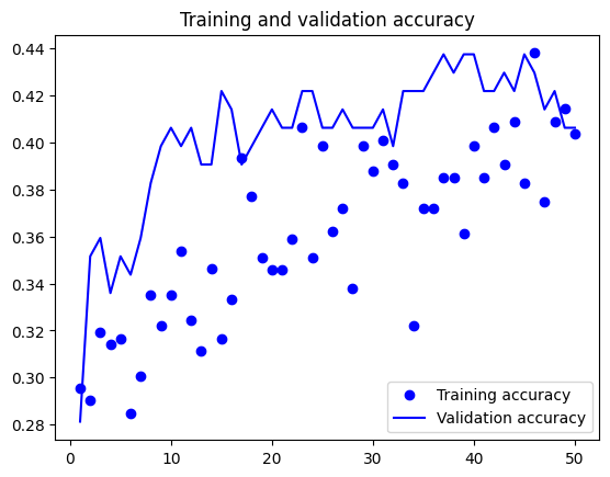
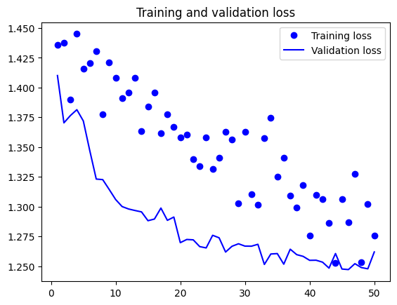
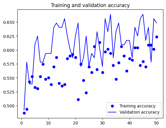
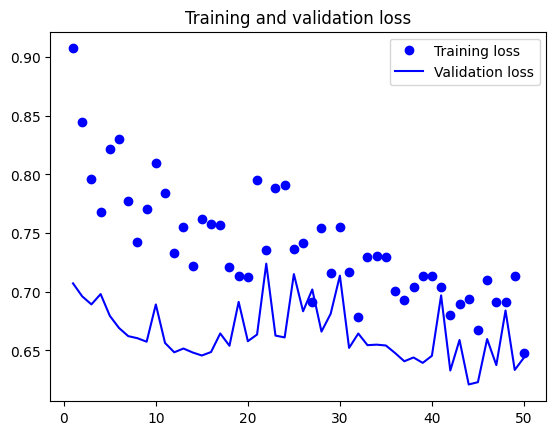
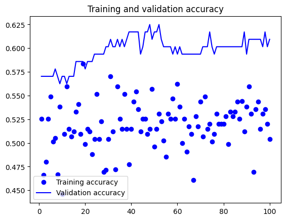
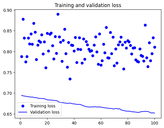
1. VGG16 model with Total params: 14,764,866, Trainable params: 50,178, with dropout and data augmentation (for 2 Classes)
#Load the VGG16 model with pre-trained weights
vgg = VGG16(input_shape=IMAGE_SIZE + [3], weights='imagenet', include_top=False)
for layer in vgg.layers:
    layer.trainable = False
# Adding custom layers on top of VGG16
x = Flatten()(vgg.output)
# adding a dropout layer to prevent overfitting
x = Dropout(0.5)(x)
# adding output layer with number of classes = len(folders)
# it is a dense (fully connected) layer with a softmax activation function
prediction = Dense(len(folders), activation='softmax')(x)
# taking the VGG16 model's input and connecting it to the custom layers added earlier for prediction.
vgg_model = Model(inputs=vgg.input, outputs=prediction)
# load best model
test_model = keras.models.load_model(
    "./models/convnet_with_just_vgg.keras")
# evaluate the model on the testset
test_loss, test_acc = test_model.evaluate(test_set)
print(f"Test accuracy: {test_acc:.3f}")
# Plotting the training loss and validation loss
# Plotting the training accuracy and validation accuracy

accuracy = history.history["accuracy"]
val_accuracy = history.history["val_accuracy"]
loss = history.history["loss"]
val_loss = history.history["val_loss"]
epochs = range(1, len(accuracy) + 1)
plt.plot(epochs, accuracy, "bo", label="Training accuracy")
plt.plot(epochs, val_accuracy, "b", label="Validation accuracy")
plt.title("Training and validation accuracy")
plt.legend()
plt.figure()
plt.plot(epochs, loss, "bo", label="Training loss")
plt.plot(epochs, val_loss, "b", label="Validation loss")
plt.title("Training and validation loss")
plt.legend()
plt.show()
2. ResNet50V2 with Total params: 23,765,506 and Trainable params: 200,706, with no dropout and with data augmentation (for 2 Classes)
# defining the model
resnet = ResNet50V2(input_shape=IMAGE_SIZE + [3], weights='imagenet', include_top=False)
for layer in resnet.layers:
    layer.trainable = False
x = Flatten()(resnet.output)
prediction = Dense(len(folders), activation='softmax')(x)
resnet_model = Model(inputs=resnet.input, outputs=prediction)
# loading the model and displaying the accuracy on the test data
test_model = keras.models.load_model(
    "./models/convnet_with_resnet.keras")
test_loss, test_acc = test_model.evaluate(test_set)
print(f"Test accuracy: {test_acc:.3f}")
accuracy = history.history["accuracy"]
val_accuracy = history.history["val_accuracy"]
loss = history.history["loss"]
val_loss = history.history["val_loss"]
epochs = range(1, len(accuracy) + 1)
plt.plot(epochs, accuracy, "bo", label="Training accuracy")
plt.plot(epochs, val_accuracy, "b", label="Validation accuracy")
plt.title("Training and validation accuracy")
plt.legend()
plt.figure()
plt.plot(epochs, loss, "bo", label="Training loss")
plt.plot(epochs, val_loss, "b", label="Validation loss")
plt.title("Training and validation loss")
plt.legend()
plt.show()
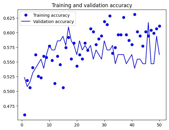
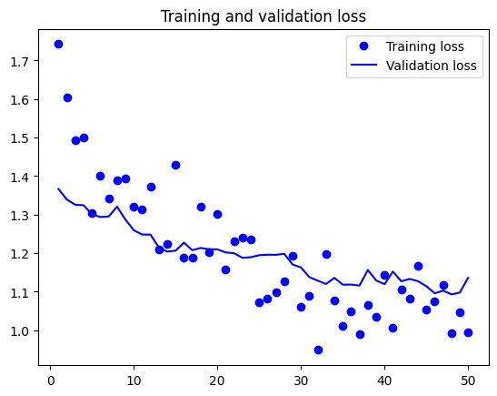
3. InceptionResNetV2 with Total params: 54,339,810 and Trainable params: 3,074, with dropout of 0.5, Global Average Pooling and a fully connect layer
# Defining the model
inception = InceptionResNetV2(weights='imagenet', include_top=False, input_shape=(299, 299, 3))

for layer in inception.layers:
    layer.trainable = False
x = inception.output
x = GlobalAveragePooling2D()(x)
x = Flatten()(x)
x = Dropout(0.5)(x)
predictions = Dense(2, activation='softmax')(x)

inception_model = Model(inputs=inception.input, outputs=predictions)
test_model = keras.models.load_model(
    "./models/convnet_with_inceptionResnet.keras")
test_loss, test_acc = test_model.evaluate(test_set)
print(f"Test accuracy: {test_acc:.3f}")
accuracy = history.history["accuracy"]
val_accuracy = history.history["val_accuracy"]
loss = history.history["loss"]
val_loss = history.history["val_loss"]
epochs = range(1, len(accuracy) + 1)
plt.plot(epochs, accuracy, "bo", label="Training accuracy")
plt.plot(epochs, val_accuracy, "b", label="Validation accuracy")
plt.title("Training and validation accuracy")
plt.legend()
plt.figure()
plt.plot(epochs, loss, "bo", label="Training loss")
plt.plot(epochs, val_loss, "b", label="Validation loss")
plt.title("Training and validation loss")
plt.legend()
plt.show()
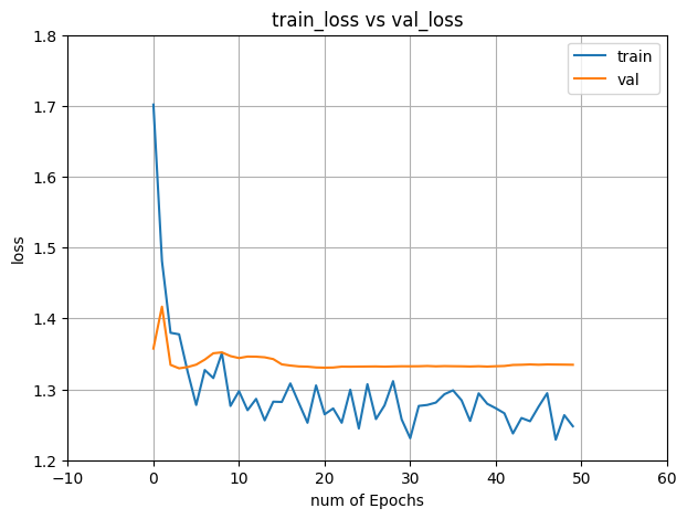
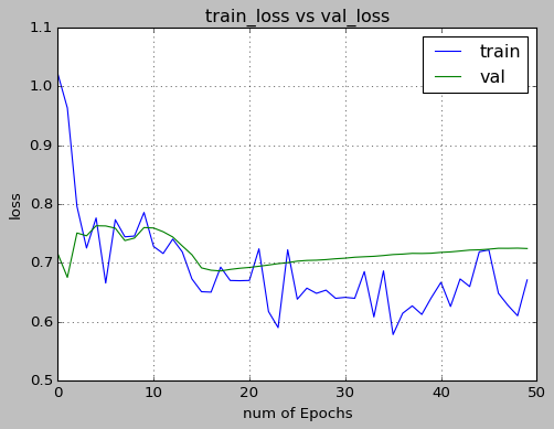
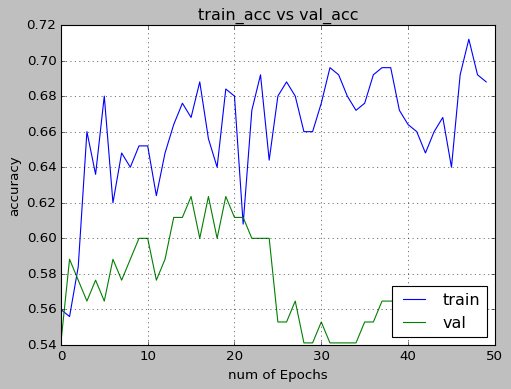
4. MobileNETV2 with Total params: 2,985,762 and Trainable params: 726,754, with dropout of 0.3, Average Pooling and a fully connected layer
tf.keras.backend.clear_session()
mnet = MobileNetV2(include_top = False, weights = "imagenet" ,input_shape=(224,224,3))
model = Sequential([mnet,
                    GlobalAveragePooling2D(),
                    Dense(512, activation = "ReLU"),
                    BatchNormalization(),
                    Dropout(0.3),
                    Dense(128, activation = "ReLU"),
                    Dropout(0.1),
                    Dense(32, activation = "ReLU"),
                    Dropout(0.3),
                    Dense(2, activation = "sigmoid")])

model.layers[0].trainable = False

model.compile(loss="categorical_crossentropy", optimizer="Adam", metrics="accuracy")

model.summary()
Model: "sequential"
Model: "sequential"
_________________________________________________________________
 Layer (type)                Output Shape              Param #
=================================================================
 mobilenetv2_1.00_224 (Funct  (None, 7, 7, 1280)       2257984
 ional)

 global_average_pooling2d (G  (None, 1280)             0
 lobalAveragePooling2D)

 dense (Dense)               (None, 512)               655872

 batch_normalization (BatchN  (None, 512)              2048
 ormalization)

 dropout (Dropout)           (None, 512)               0

 dense_1 (Dense)             (None, 128)               65664

 dropout_1 (Dropout)         (None, 128)               0

 dense_2 (Dense)             (None, 32)                4128

 dropout_2 (Dropout)         (None, 32)                0

 dense_3 (Dense)             (None, 2)                 66

=================================================================
Total params: 2,985,762
Trainable params: 726,754
Non-trainable params: 2,259,008
_________________________________________________________________
test_loss, test_accuracy = model.evaluate_generator(generator = test_set, verbose = 1)

print('Test Accuracy: ', round((test_accuracy * 100), 2), "%")
epochs = 50
train_loss = hist.history['loss']
val_loss = hist.history['val_loss']
train_acc = hist.history['accuracy']
val_acc = hist.history['val_accuracy']
xc = range(epochs)
plt.figure(1,figsize=(7,5))
plt.plot(xc,train_loss)
plt.plot(xc,val_loss)
plt.xlabel('num of Epochs')
plt.ylabel('loss')
plt.title('train_loss vs val_loss')
plt.grid(True)
plt.legend(['train','val'])
#print plt.style.available # use bmh, classic,ggplot for big pictures
plt.style.use(['classic'])
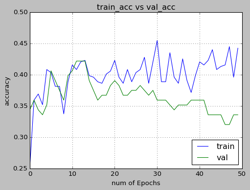
plt.figure(2,figsize=(7,5))
plt.plot(xc,train_acc)
plt.plot(xc,val_acc)
plt.xlabel('num of Epochs')
plt.ylabel('accuracy')
plt.title('train_acc vs val_acc')
plt.grid(True)
plt.legend(['train','val'],loc=4)
#print plt.style.available # use bmh, classic,ggplot for big pictures
plt.style.use(['classic'])
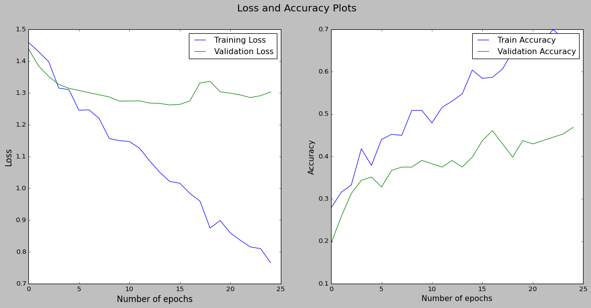
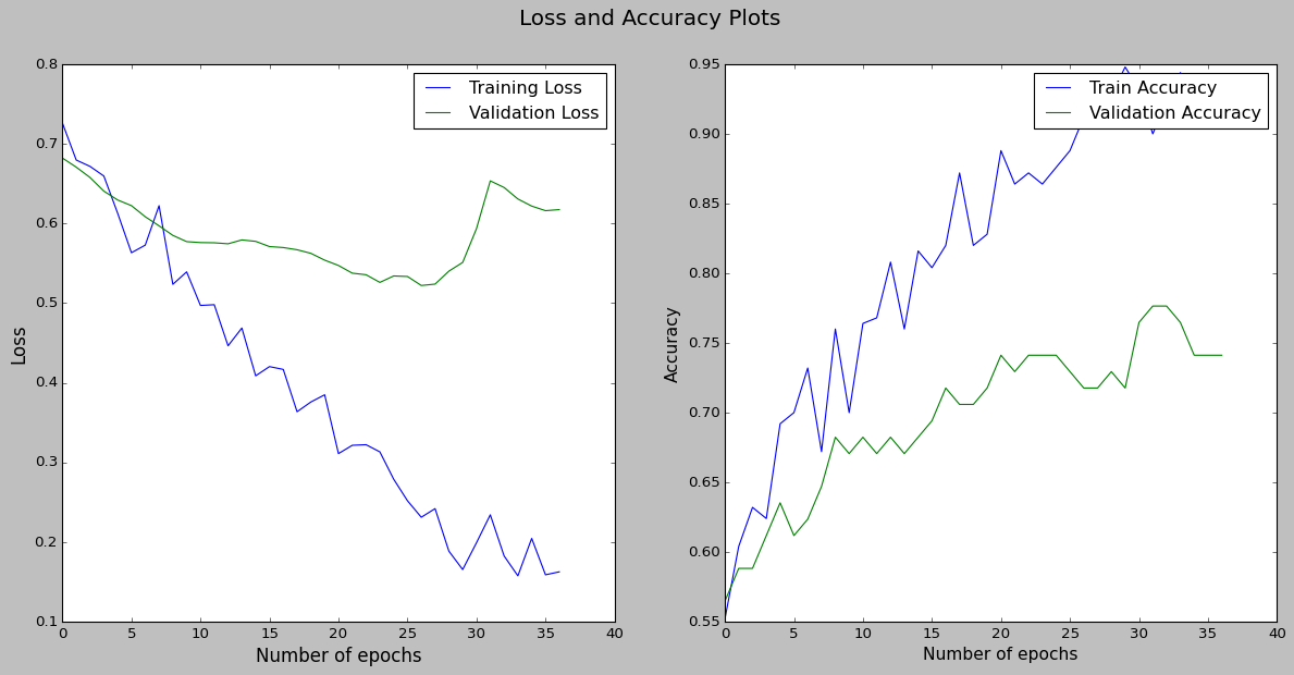
5. EfficientNET with Total params: 4,052,126 and Trainable params: 4,010,110, with dropout of 0.5, GlobalAveragePooling and a fully connected layer
efnb0 = efn.EfficientNetB0(weights='imagenet', include_top=False, input_shape=(224,224,3), classes=n_classes)

model = Sequential()
model.add(efnb0)
model.add(GlobalAveragePooling2D())
model.add(Dropout(0.5))
model.add(Dense(n_classes, activation='softmax'))

model.summary()
Model: "sequential_1"
_________________________________________________________________
 Layer (type)                Output Shape              Param #
=================================================================
 efficientnet-b0 (Functional  (None, 7, 7, 1280)       4049564
 )

 global_average_pooling2d_1   (None, 1280)             0
 (GlobalAveragePooling2D)

 dropout_3 (Dropout)         (None, 1280)              0

 dense_4 (Dense)             (None, 2)                 2562

=================================================================
Total params: 4,052,126
Trainable params: 4,010,110
Non-trainable params: 42,016
_________________________________________________________________
test_loss, test_accuracy = model.evaluate_generator(generator = test_set, verbose = 1)

print('Test Accuracy: ', round((test_accuracy * 100), 2), "%")
/var/folders/qn/c0ll_4m107d0w2b21m8wkgz80000gn/T/ipykernel_1833/1841467748.py:1: UserWarning: `Model.evaluate_generator` is deprecated and will be removed in a future version. Please use `Model.evaluate`, which supports generators.
  test_loss, test_accuracy = model.evaluate_generator(generator = test_set, verbose = 1)


1/1 [==============================] - 0s 230ms/step - loss: 0.5937 - accuracy: 0.5312
Test Accuracy:  53.12 %
#plot to visualize the loss and accuracy against number of epochs
plt.figure(figsize=(18,8))

plt.suptitle('Loss and Accuracy Plots', fontsize=18)

plt.subplot(1,2,1)
plt.plot(model_history.history['loss'], label='Training Loss')
plt.plot(model_history.history['val_loss'], label='Validation Loss')
plt.legend()
plt.xlabel('Number of epochs', fontsize=15)
plt.ylabel('Loss', fontsize=15)

plt.subplot(1,2,2)
plt.plot(model_history.history['accuracy'], label='Train Accuracy')
plt.plot(model_history.history['val_accuracy'], label='Validation Accuracy')
plt.legend()
plt.xlabel('Number of epochs', fontsize=14)
plt.ylabel('Accuracy', fontsize=14)
plt.show()
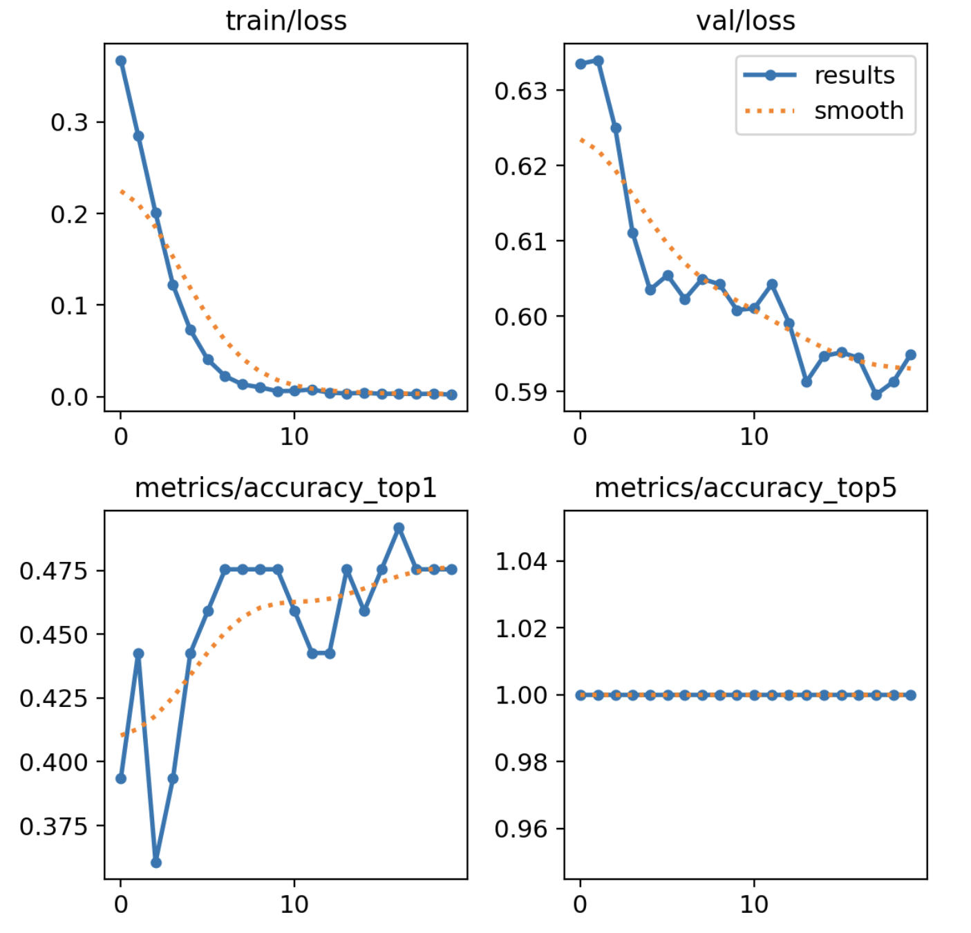
6. YoloV8 with 99 layers, 1440850 parameters, 1440850 gradients
model = YOLO('yolov8n-cls.pt') # load a pretrained model (recommended for training)
# Train the model
model.train(data='/home/jorgeluisg/Documents/001_George_brown/DL_2/project/data', epochs=20, imgsz=64)
# Predict with the model
results = predict(source)  # predict on an image

Model Results
| Model VS Accuracy | With 4 classes | With 2 classes |
|---|---|---|
| VGG 16 | 34.4% | 63.3% |
| ResNet50V2 | 31.1% | 56.7% |
| InceptionResNetV2 | 34.4% | 60% |
| MobileNETV2 | 25% | 65.62% |
| EfficientNET | 31.67% | 53.12% |
| YOLO V8 | 47.5% | 75% |
Conclusion
We looked at different image classification models like VGG, ResNet50, InceptionResNetV2, MobileNetV2, EfficientNetB0, and YOLOv8. We had a tough time because the classes we were trying to classify, like kick, punch, kicknt, and punchnt, were very similar. Surprisingly, when we tried to improve accuracy by adding dropout (a technique to prevent overfitting), it didn’t help much and our accuracy stayed around 30%, even with data augmentation. So, we decided to focus only on the kick and punch classes. This made a big difference, and our accuracy improved by 30% across all models!
Then, we tried a model called YOLOv8n, comparing the original dataset with all four classes to a simpler one with just kick and punch. YOLOv8n consistently gave better accuracy with the simplified dataset, showing that it’s the best choice for our specific task.